Discriminant Function

The purpose of a discriminant function analysis is to predict group membership based on a linear combination of the interval variables. The procedure begins with a set of observations where both group membership and the values of the interval variables are known. The end result of the procedure is a model that allows prediction of group membership when only the interval variables are known. Another purpose of discriminant function analysis is an understanding of the data set, as a careful examination of the prediction model that results from the procedure can give insight into the relationship between group membership and the variables used to predict group membership.

Discriminant analysis is used when:

• The dependent is categorical with the predictor IV’s at interval level such as age, income, attitudes, perceptions, and years of education, although dummy variables can be used as predictors as in multiple regression. Logistic regression IV’s can be of any level of measurement.

• There are more than two DV categories, unlike logistic regression, which is limited to a dichotomous dependent variable.

Discriminant analysis involves the determination of a linear equation like regression that will predict which group the case belongs to. The form of the equation or function is:

D=v1XI + v2X2 + v3X3.....

=viXi + a

Where D = discriminate function

v = the discriminant coefficient or weight for that variable

X = respondent’s score for that variable

a = a constant

i = the number of predictor variables

Purpose of Discriminant analysis:

• To investigate differences between groups on the basis of the attributes of the cases, indicating which attributes contribute most to group separation. The descriptive technique successively identifies the linear combination of attributes known as canonical discriminant functions (equations) which contribute maximally to group separation.

• Predictive DA addresses the question of how to assign new cases to groups. The DA function uses a person’s scores on the predictor variables to predict the category to which the individual belongs.

• To determine the most parsimonious way to distinguish between groups.

• To classify cases into groups. Statistical significance tests using chi square enable you to see how well the function separates the groups.

• To test theory whether cases are classified as predicted

The aim of the statistical analysis in DA is to combine (weight) the variable scores in some way so that a single new composite variable, the discriminant score, is produced.

Posted by

Amit Kulkarni

Finance

Learnings from Business Analytics

Business Analytics focuses on identifying the changes to an organization that are required to achieve strategic goals.These include changes in strategy , structure, processes , policy and information system.

It focuses on understanding the needs of the business as a whole , its strategic direction and identifying initiative that will help make those strategies into goals.

It includes creating and maintaining business architecture , feasibility studies , identifying new business opportunities, preparing business case and conducting the initial risk assessment.

Here I try to sum up what I have learnt till now in the BA course.

Factor analysis

Factor analysis is a collection of methods used to examine how constructs influence the responses on a number of measured variables.

Measures that are highly correlated are likely influenced by the same factors while measures that are not highly correlated are likely uninfluenced by different factors.

Factor analysis has its application in various fields like economics (to get important factors which affect the economy) , Behavioural Analysis(What are the important factors impacting the human

Behaviour), Marketing(What are the major factors impacting the decision of a consumer to select a specific brand.

It can also be used in market research. Market research data can be factored to understand the results more clearly.

Discriminant Analysis:

It is most often used to help a researcher predict the group in which a subject belongs.

The predictor variable needs to be ordinal or scale, which helps us analyze the effect of such variables on our hypothesis. The most famous application of this method is bankruptcy prediction where Altman z score is used which tells us whether a firm will survive or not.

Conjoint Analysis:

It applies a complex form of analysis of variance to the data obtained from each respondent.

Then it calculates the value for each feature. Features with the highest value are judged the most important to respondents. It tries to identify the interdependency existing between a no. of variables.

It can be used to investigate the attributes that influence individual investors decision making process to buy shares. It also tells us how people make choices between products or services, so that companies can design new products or service meeting customer needs.

Cluster Analysis:

K-means clustering:

It is an algorithm for clustering data that allows the user to choose the number of clusters one would like to have from a given set , based on some similarity.

With a large data set K-means is faster than hierarchical clustering. Data reduction is accomplished by replacing the co-ordinates of each point on a cluster with the cluster’s centroid.

K-means can be helpful for a bank , which is looking at analysing customers in the corporate world on who to target and how much loan to offer to which kind of customers. K-means clustering can be used to find the ideal company with the best risk –return profile using the ratios( like cash , inventory turnover, ROE, ROA) and then cluster of companies around the ideal company can be created. All the companies in that cluster can then be suitable for the bank.

Hierarchical clustering:

Hierarchical clustering is nothing but grouping of data on various scales. Usually a cluster tree is created , which is also known as a dendrogram. In dendrograms, the first step is to find which elements should be merged in a cluster. For the same purpose, two elements which are closest are taken and the same process gets repeated.

Posted by

Neeraj Singh

Finance

Revision: Factor Analysis!!

Factor Analysis - Geometric Model

An understanding of the patterns defined by factor analysis can be enhanced through a geometric interpretation. Each nation can be thought of as defining a coordinate axis of a geometric space. For example, the US, the UK, and the

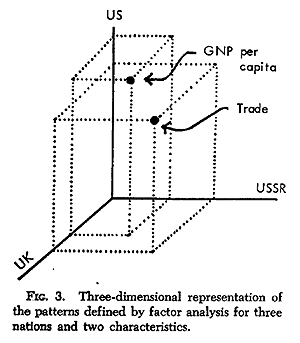
USSR can define a three

-dimensional space as given in Figure 3. Imagine that the axis for the UK is projecting at right angles from the paper. Although pictorially constrained to three dimensions, the space can be analytically extended to fourteen dimensions at right angles to each other and thus represent the fourteen nations.

Now, in this space each characteristic can be con

sidered a point located according to its value for each nation. Such a plot is shown in Figure 3 for the GNP per capita and trade values of the US, UK, and USSR. To make the plot explicit, projections for each point are drawn as dotted lines to each axis.

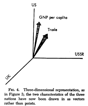
If for each point in Figure 3 we draw a line from the origin to the point and top the line off with an arrowhead as shown in Figure 4, then we have a vector representation of the data. The characteristics of similarly plotted as vectors in an imaginary space of the fourteen nations (dimensions) would describe a vector space. In this space, consider two vectors representing any two of these characteristics for the fourteen nations.

The angle between these vectors measures the relationship between the two characteristics for the fourteen nations. The closer to 90^o the angle is, the less the relationship is. If two vectors are at a right angle, the characteristics they represent are uncorrelated: they have no relationship to each other. In other words, some nations will be high on one characteristic, say GNP per capita, and low on the other, say trade; some nations will be low on GNP per capita and high on trade; some nations will be high on both, and some will be low on both. No regularity exists in their covariation.

The closer the angle between the vectors is to zero, the stronger the relationship between the characteristics. An angle of zero means that nations high or low on one characteristic are proportionately high or low on the other. Obtuse angles mean a negative relationship. At the extreme, an angle of 180^o between two vectors means that the two characteristics are inversely related: a nation high on one characteristic is proportionately low on the other.

Let the characteristics be projected in the fourteen-dimensional space defined by the fourteen nations as suggested in Figure 5(a). The configuration of vectors will then reflect the data interrelationships. Characteristics that are highly interrelated will cluster together; characteristics that are unrelated will be at right angles to each other. By inspecting the configuration we can discern the distinct clusters of vectors (if such clusters exist), and these clusters index the patterns of relationship in the data: each cluster is a pattern.

Were we dealing with characteristics of two or three nations, patterns could be found by simply plotting the characteristics as vectors. What factor analysis does geometrically is this: it enables the clusters of vectors to be defined when the number of cases (dimensions) exceeds our graphical limit of three. Each factor delineated by factor analysis defines a distinct cluster of vectors.

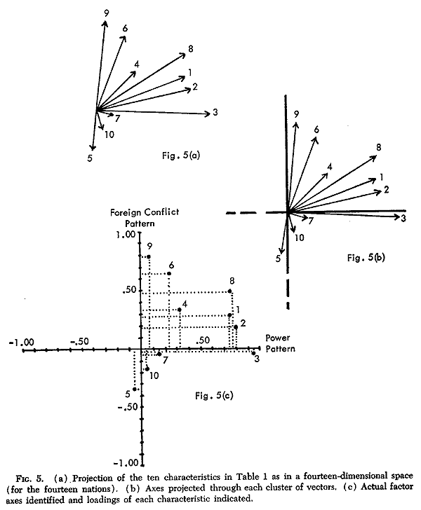
Consider Figure 5(a) again. Factor analysis would mathematically lay out such a plot and then project an axis through each cluster as shown in Figure 5(b). This is analogous to giving each vector point in a cluster a mass of one and letting the factor axes fall through their center of gravity. The projection of each vector point on the factor axes defines the clusters. These projections are called loadings and the factor axes are often called factors or dimensions.

Figure 5(c) pictures the power and foreign conflict patterns. For simplicity, the configuration of points is shown, rather than vectors, and the two factor axes are indicated (as actually derived from a factor analysis). The loadings of each characteristic (i.e., each point in space) on each axis are also displayed. This figure may clarify how factor loadings as a set of numbers can define

• a pattern of relationships and
• the association of each characteristic with each pattern.

Author – Ankit Gupta

Marketing Group 1

CHOOSING A WIFE USING CONJOINT ANALYSIS!!!

Inspired by the last few lectures of Business Analytics, I thought to come up with a story of how a man can use Conjoint Analysis in the process of arrange marriages and get himself the most suitable wife.

So the story goes like this...

After a lot of persistence from his parents, Dhruv agreed to start looking for a suitable girl for marriage. But he was not sure as to how would he be able to know if the girl was “perfect” for him. He was looking for a guaranteed method that he could use in the process.

Just a day before he was about to start meeting girls, he miraculously got what he was looking for. During his Business Analytics class he was taught Conjoint Analysis. Conjoint Analysis is a market research technique in which consumers make tradeoffs between two or more features and benefits of a product on a scale ranging from 'Most Preferred' to 'Least Preferred.' coupled with techniques such as simulation analysis, conjoint analysis helps in evaluation of different points.

Just during this lecture, Dhruv got an idea that by using Conjoint Analysis he could cut down on meeting all the 15 girls his mother wanted him to meet. Right after the class he prepared a list of possible attributes that he wanted in his life partner. The list contained things like looks, family background, intelligence, occupation, education, household skills etc. After putting all the attributes and the options for each attribute, (for e.g. Attribute – looks, Options – Very good looking, good looking, average) he came up with all the permutations and combinations possible.

Once his list was final, he sat with his mom to discuss what all attributes that every girl had. He prepared an excel sheet with all the data he collected. Now the next step was to rate all the girls out of 10 on the attributes that were similar to his dream girl. During the rating only, he was sure that he didn’t want to meet 8 girls as they were not at all compatible with him. Once the rating was done, he put the data in SPSS and analyzed it. Now after analyzing the data, he came to know what all factors were more important to him than the others. Now he was sure about what attributes to look for in the girls he would meet.

Now was the most important thing – look for the attributes in the girls. One by one he met the remaining 7 females and analyzed them on the attributes that were most important to him. In less than 4 days he had met all the 7 girls and now he had to see who fit the bill the most. Some of them were close to what he was looking for and some of them missed the target by a mile. He finally shortlisted 2 girls (both of them were ranked 10 by him earlier) that he thought were the closest to what he wanted. He thanked his Conjoint Analysis and SPSS software to make his task so much simpler. The software had done its job; it would be of no help any further.

Now Dhruv will have to trust his instincts and GOD to get his soul mate. Tomorrow he will be meeting both the girls once more and then decide who would he want as his wife. Let’s all of us wish him all the best for one of the most important decision of his life.

Written by: Ajvad Rehmani

Group: 13003

Perceptual Analysis on " FlitterIn"

Objective : of this blog post is to study in very simple terms how the three stalwarts of the social media space – Facebook, Twitter and Linkedin are perceived by a common user.

Purpose : of carrying out this analysis is to debate whether there

· is a gap in the respective company’s desired positioning vis-à-vis the actual perception

· are gaps that the new entrants like Google Buzz or Google Me can exploit.

Method : Perceptual Mapping are easy to interpret graphs that visually display the perceptions of customers about a brand. I have used this

technique to display the relative position of Facebook, Twitter and Linkedin across certain key attributes.

Before we embark upon the analysis, it is important to put in perspective certain key stats about the three companies.

Analysis by way of Perceptual Maps

Perceptual Map 1 : Personal Vs Professional Networking

· Facebook scores very high on personal networking but low on professional networking.

· Facebook users tend to look for and interact more with old friends/acquaintances.

· Twitter has much better use of professional networking with corporate in the fray too.

· Twitter users are more open to making new friends – who had been total strangers till they met on Twitter.

· Linkedin’s perception is that of a business/professional networking site. That’s how it has been officially positioned as well.

Perceptual Map 2 : Knowledge Based Vs Relationship Based Updates

Twitter scores the highest in knowledge based updates. This includes links to news, opinions and blogs.

· Personal updates on Twitter are not that common. In fact, they are despised, with a threat of unfollowing looming large in case they are used more often.

· Linkedin is low on updates of any kind. That’s something Linkedin management is trying to address through measures like provision for article links, the ‘like’ button etc.

· Facebook is high on personal updates but low on knowledge based ones.

·

Perceptual Map 3 : Privacy Vs Downtime

· Linkedin has neither faced privacy issues nor any serious downtimes.

· Twitter is pathetic in terms of downtime.

· Twitter has also faced privacy issues, with the hacking menace giving jitters to users every now and then.

· However, since Twitter has been positioned as an open/public site, too much personal information is neither desired nor available on the website that could cause any serious privacy issue.

· Facebook is facing serious privacy issues but seems to be doing fine as far is downtime is concerned.

Conclusion

There are sufficient gaps in the social media space that Google can exploit, viz

· Perceptual Map 1 : There is no website that is high on both professional and personal updates at the same time. Is this an opportunity for Google, or an invitation to confused positioning?

· Perceptual Map 3 : Can Google Me offer excellent privacy with minimal downtime? Google is a powerhouse, and can achieve both! (Only if it does not botch up accidentally as it did with Google Buzz!)

As per Perceptual Map 2, both twitter and Facebook are comfortably placed in their respective quadrants, and it would be difficult to nudge past them!

Disclaimer – These maps are based on my perceptions of the three companies.

Author:- Lincy Thomas

Group:- Operations 3

Conjoint Analysis

Conjoint Analysis is a procedure for measuring, analyzing, and predicting customer’s responses to new products and to new features of existing products. It enables companies to fester customer’s preferences for products into part-worth utilities associated with each option of each attribute or feature of the product category. Companies can then recombine the part-worth to predict customer’s preferences for any combination of attribute options, to determine the optimal product concept or to identify market segments that value a particular product concept highly.

Factors and their values are defined by the researcher in advance. The various combinations of the factor values yield fictive products that are being ranked by the interviewed persons. With Conjoint Analysis it is possible to derive metric partial utilities from the ranking results. The summation of these partial utilities therefore results in metric total utilities.

Conjoint Analysis

· Independent variables: Object attributes.

· Dependent variable: Preferences of the interviewed person for the fictive products.

· The utility structure of a number of persons can be computed through aggregation of the single results.

Conjoint Analysis

· Factors and Factor Values

o Important for the choice of factors and their values are

§ Relevance

§ Interference

§ Independence

§ Realisable

§ Compensatory relationships of the various factor values

§ They do not constitute exclusion criteria

§ Terminable

Conjoint Analysis

Possibilities of rating of the incentives

· Ranking

· Rough classifications into groups of different utility with succeeding ranking within these groups.

· Aggregation of these results leads to a total ranking. Used when there are a large number of incentives.

· Rating scales

· Paired comparison

Conjoint Analysis

Estimation of the utility values

Conjoint Analysis is used to determine partial utilities (partworths) for all factor values based upon the ranked data. Furthermore, with this partworths it is possible to compute the metric total utilities of all incentives and the relative importance of the single object attributes.

Individual Conjoint Analysis: For each person utility values are computed.

Combined Conjoint Analysis: Only one value for each factor category.

Conjoint Analysis

Estimation of the utility values of target criterion for the determination of the partial utilities:

The resulting total utilities should yield a good representation of the empirically ranked data. Related procedure for the determination of the partial utilities: monotonous analysis of variance.

Author:- Ishan Tupe

Group :- Operations 3

REGRESSION

Rather than discussing about the various methods taught in class, I thought today I’ll review some of the facts related to regression; which is the basic knowledge required to draw conclusions from the output of the “Discriminant Analysis”.

Regression analysis is used to produce an equation that will predict a dependent variable using one or more independent variables. This equation has the form

Y = b1X1 + b2X2 + ... + A

where Y is the dependent variable being predicted;

X1, X2 and so on are the independent variables being used to predict it;

b1, b2 and so on are the coefficients or multipliers that describe the size of the effect the independent variables are having on the dependent variable Y, and

A is the value Y is predicted to have when all the independent variables are equal to zero.

Suppose we have a regression equation for the dependent variable,

PRICE = -294.1955 (mpg) + 1767.292 (foreign) + 11905.42; telling us that price is predicted to increase by 1767.292 when the foreign variable goes up by one, decrease by 294.1955 when mpg goes up by one, and is predicted to be 11905.42 when both mpg and foreign are zero.

Coming up with a prediction equation like this is useful, only if the independent variables in the dataset have some correlation with the dependent variable. So in addition to the prediction components of our equation--the coefficients on our independent variables (betas) and the constant (alpha)--we need some measure to tell us how strongly each independent variable is associated with our dependent variable.

When running the regression model, we are trying to discover whether the coefficients on our independent variables are really different from 0 (so the independent variables are having a genuine effect on our dependent variable) or if alternatively any apparent differences from 0 are just due to random chance. The null (default) hypothesis is always that each independent variable is having absolutely no effect (has a coefficient of 0) and we are looking for a reason to reject this theory.

Coefficients

In simple or multiple linear regression, the size of the coefficient for each independent variable gives the magnitude of the effect that variable is having on the dependent variable, and the sign on the coefficient (positive or negative) gives the direction of the effect. In regression with a single independent variable, the coefficient tells how much the dependent variable is expected to increase (if the coefficient is positive) or decrease (if the coefficient is negative) when that independent variable increases by one. In regression with multiple independent variables, the coefficient tells how much the dependent variable is expected to increase when that independent variable increases by one, holding all the other independent variables constant. We would have to keep in mind the units which our variables are measured in.

R-Squared and overall significance of the regression

The R-squared of the regression is the fraction of the variation in the dependent variable that is accounted for (or predicted by) the independent variables. (In regression with a single independent variable, it is the same as the square of the correlation between your dependent and independent variable.)

With this blog, I hope to have covered some of the intrinsic underlying facts behind the regression model and its analysis.

Posted by-

EMI JAVAHARILAL (13134)

Operations Group 2